Introduction
This vignette walks users through the mechanics of the functions and workflows that produce all of the Reporting output within the gsm package. gsm leverages Key Risk Indicators (KRIs) and thresholds to conduct study-level, country-level and site-level Risk Based Monitoring for clinical trials.
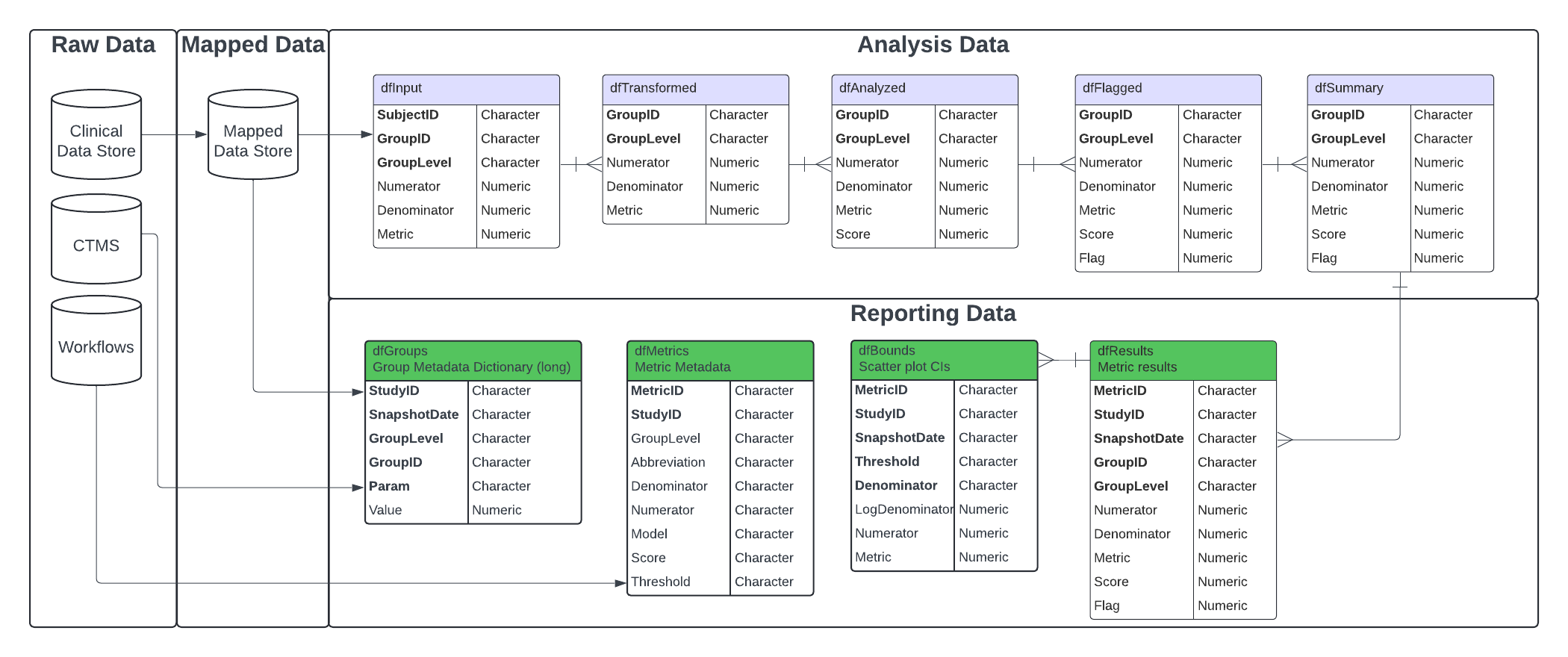
These functions and workflows produce data frames, visualizations, metadata, and reports to be used in reporting and error checking at clinical sites. The image below illustrates the overarching context in which the reporting workflow runs, taking inputs from both the output of the analytics workflow, as well as raw study-, site-, and country-level data in the Raw/Raw+ format.
All of the functions to create the data frames in the reporting data
model will run automatically and sequentially when a user specifies the
metadata and data needed for the report, and calls upon the
RunWorkflow() function on the yaml files in the
workflow/3_reporting directory. To create a report, the
output of the reporting yamls is fed into the yamls in the
workflow/4_modules directory to produce and html document
with all charts and tables created in the reporting workflow. For a more
detailed discussion of the yaml file and directory structure, see
(vignette("gsmExtensions")).
Each of the individual functions can also be run independently outside of a specified yaml workflow.
For the purposes of this documentation, we will evaluate the input(s) and output(s) of each individual function for a specific KRI to show the stepwise progression of how a yaml workflow is set up to handle and process reporting-level data.
Case Study - Step-by-Step Full Site-Level Report
We will use sample clinical data from the {clindata}
package to run the full site-level report for all 12 KRIs included in
this package. The focus of this vignette is the reporting workflow, so
the output of the analytics workflow will be briefly discussed, but only
in the context of inputs to the reporting workflow.
Additional supporting functions are explored in Appendix 1.
Step 0 - Run Analysis Workflow(s)
Prior to running the reporting model to create reporting data frames,
charts and reports, the metrics we are reporting on must be properly
calculated and flagged with the analysis workflow. For more information
on the Analysis Workflow, see the associated
vignette("DataAnalysis").
To run the analysis workflow on all 13 KRIs using
clindata Raw+ data, use the code snippet below. From this,
three pieces of output will be used in the reporting workflow:
-
lAnalysis- list of data frames in the analysis data model -
lWorkflow- list containing the metadata for each of the KRIs -
mapped$Mapped_ENROLL- mapped data.frame of enrolled participants
# Create Mapped Data - filter/map raw data
lSource <- list(
    Source_SUBJ = clindata::rawplus_dm,
    Source_AE = clindata::rawplus_ae,
    Source_PD = clindata::ctms_protdev,
    Source_LB = clindata::rawplus_lb,
    Source_STUDCOMP = clindata::rawplus_studcomp,
    Source_SDRGCOMP = clindata::rawplus_sdrgcomp %>% dplyr::filter(.data$phase == 'Blinded Study Drug Completion'),
    Source_DATACHG = clindata::edc_data_points,
    Source_DATAENT = clindata::edc_data_pages,
    Source_QUERY = clindata::edc_queries,
    Source_ENROLL = clindata::rawplus_enroll,
    Source_SITE = clindata::ctms_site,
    Source_STUDY = clindata::ctms_study
)

# Step 0 - Data Ingestion - standardize tables/columns names
mappings_wf <- MakeWorkflowList(strPath = "workflow/1_mappings")
mappings_spec <- CombineSpecs(mappings_wf)
lRaw <- Ingest(lSource, mappings_spec)

# Step 1 - Create Mapped Data Layer - filter, aggregate and join raw data to create mapped data layer
mapped <- RunWorkflows(mappings_wf, lRaw)

# Step 2 - Create Metrics - calculate metrics using mapped data
metrics_wf <- MakeWorkflowList(strPath = "workflow/2_metrics", strNames = "kri")
lAnalysis <- RunWorkflows(metrics_wf, mapped)
Step 1 - Create Reporting Model Data Frames
With all necessary inputs to the reporting model created, we can move on to generate the reporting data model data frames. These data frames created are as follows:
-
dfGroups: Group-level metadata dictionary. Created by passing CTMS site and study data toMakeLongMeta(). -
dfMetrics: Metric-specific metadata for use in charts and reporting. Created by passing anlWorkflowobject toMakeMetric(). -
dfResults: A stacked summary of analysis pipeline output. Created by passing a list of results returned bySummarize()toBindResults(). -
dfBounds: Set of predicted percentages/rates and upper- and lower-bounds across the full range of sample sizes/total exposure values for reporting. Created by passingdfResultsanddfMetricstoMakeBounds().
For more details on any of these tables, see
vignette("DataModel").
The following sub-steps will dive into the creation and structure of
each of these tables. Sample data for each of these tables can found in
gsm as reportingGroups,
reportingMetrics, reportingResults and
reportingBounds. These sample tables are used throughout
the package in examples and documentation.
Step 1.1 - Transform CTMS data into dfGroups data
frame
The dfGroups data frame is critical to providing site-,
study- and country-level information in the final report. This table is
based on CTMS data and the mapped Mapped_SUBJ data frame
created in the Mapping workflow. Creating this table requires the
creation of 5 smaller tables that summarize the data at each group level
using RunQuery() and MakeLongMeta(). These
small tables are then bound together to create
dfGroups.
#Transform CTMS Site and Study Level data
dfCTMSSite <- RunQuery(df = clindata::ctms_site,
                       strQuery = "SELECT pi_number as GroupID, site_status as Status, pi_first_name as InvestigatorFirstName, pi_last_name as InvestigatorLastName, city as City, state as State, country as Country, * FROM df") |>
  MakeLongMeta(strGroupLevel = 'Site')

dfCTMSStudy <- RunQuery(df = clindata::ctms_study,
                        strQuery = "SELECT protocol_number as GroupID, status as Status, * FROM df") |>
  MakeLongMeta(strGroupLevel = 'Study')

# Get Participant and Site counts for Country, Site and Study
dfSiteCounts <- RunQuery(df = mapped$Mapped_SUBJ,
                             strQuery = "SELECT invid as GroupID, COUNT(DISTINCT subjid) as ParticipantCount, COUNT(DISTINCT invid) as SiteCount FROM df GROUP BY invid") |>
  MakeLongMeta(strGroupLevel = "Site")

dfStudyCounts <- RunQuery(df = mapped$Mapped_SUBJ,
                             strQuery = "SELECT studyid as GroupID, COUNT(DISTINCT subjid) as ParticipantCount, COUNT(DISTINCT invid) as SiteCount FROM df GROUP BY studyid") |>
  MakeLongMeta(strGroupLevel = "Study")

dfCountryCounts <- RunQuery(df = mapped$Mapped_SUBJ,
                             strQuery = "SELECT country as GroupID, COUNT(DISTINCT subjid) as ParticipantCount, COUNT(DISTINCT invid) as SiteCount FROM df GROUP BY country") |>
  MakeLongMeta(strGroupLevel = "Country")


# Combine CTMS and Counts data as dfGroups
dfGroups <- dplyr::bind_rows(SiteCounts = dfSiteCounts,
                      StudyCounts = dfStudyCounts,
                      CountryCounts = dfCountryCounts,
                      Site = dfCTMSSite,
                      Study = dfCTMSStudy)
The resulting dfGroups dataframe contains the following
columns:
-
GroupID: Group Identifier -
GroupLevel: Type of Group specified inGroupID(Country, Site, Study) -
Param: Parameter Name (e.g. “Status”)
-
Value: Parameter Value (e.g. “Active”)
A more detailed explanation of the Params for each group
level can be found in vignette("DataModel").
Step 1.2 - Create dfMetrics Metadata
The dfMetrics table contains the metadata for each of
the KRIs in the report. This information comes from the
meta section of the metric workflows,
metrics_wf defined in Step 0. Using this workflow
information as the input, MakeMetric() is used to produce a
data frame with one row per metric.
dfMetrics <- MakeMetric(lWorkflows = metrics_wf)The resulting dfMetrics dataframe contains the following
columns:
-
File: The yaml file for workflow -
MetricID: ID for the Metric -
Group: The group type for the metric (e.g. “Site”) -
Abbreviation: Abbreviation for the metric -
Metric: Name of the metric -
Numerator: Data source for the Numerator -
Denominator: Data source for the Denominator -
Model: Model used to calculate metric -
Score: Type of Score reported -
Threshold: Thresholds to be used for bounds and flags
Step 1.3 - Stack dfSummary data into
dfResults
The reporting workflow requires that all metrics are stacked into a
single data frame, dfResults. This stacked data frame is
created by feeding the lAnalysis list from the analysis
workflow into BindResults() along with the snapshot date
and the study id.
dfResults <- BindResults(lAnalysis = lAnalysis,
                         strName = "Analysis_Summary",
                         dSnapshotDate = Sys.Date(),
                         strStudyID = "ABC-123")
The resulting dfResults data frame contains the
following columns:
-
GroupID: Group Identifier -
GroupLevel: Type of Group specified inGroupID(Country, Site, Study) -
Numerator: The calculated numerator value -
Denominator: The calculated denominator value
-
Metric: The calculated rate/metric value -
Score: The calculated metric score -
Flag: The calculated flag -
MetricID: The Metric ID -
StudyID: The Study ID -
SnapshotDate: The Date of the snapshot
Step 1.4 - Create dfBounds for Confidence
Intervals
Several of the charts created for the KRI reports use confidence
intervals and bounds to delineate the observations based on the flag
they receive (no flag, amber or red). In order to create the data frame
that contains the information about these boundaries,
dfBounds, dfResults and dfMetrics
is fed into the MakeBounds() function. The
MakeBounds() function is a wrapper around the
Analyze_*_PredictBounds() functions that create the bounds
based on the model used to estimate the metric(Normal Approximation or
Poisson).
dfBounds <- MakeBounds(dfResults = dfResults,
                        dfMetrics = dfMetrics)
#> Creating stacked dfBounds data for strMetrics
#> Parsed -2,-1,2,3 to numeric vector: -2, -1, 2, 3
#> nStep was not provided. Setting default step to 203.584.
#> Parsed -2,-1,2,3 to numeric vector: -2, -1, 2, 3
#> nStep was not provided. Setting default step to 203.584.
#> Parsed -3,-2,2,3 to numeric vector: -3, -2, 2, 3
#> nStep was not provided. Setting default step to 203.584.
#> Parsed -3,-2,2,3 to numeric vector: -3, -2, 2, 3
#> nStep was not provided. Setting default step to 203.584.
#> Parsed -3,-2,2,3 to numeric vector: -3, -2, 2, 3
#> nStep was not provided. Setting default step to 121.068.
#> Parsed -3,-2,2,3 to numeric vector: -3, -2, 2, 3
#> nStep was not provided. Setting default step to 0.272.
#> Parsed -3,-2,2,3 to numeric vector: -3, -2, 2, 3
#> nStep was not provided. Setting default step to 0.272.
#> Parsed -3,-2,2,3 to numeric vector: -3, -2, 2, 3
#> nStep was not provided. Setting default step to 433.42.
#> Parsed -3,-2,2,3 to numeric vector: -3, -2, 2, 3
#> nStep was not provided. Setting default step to 8.652.
#> Parsed -3,-2,2,3 to numeric vector: -3, -2, 2, 3
#> nStep was not provided. Setting default step to 50.716.
#> Parsed -3,-2,2,3 to numeric vector: -3, -2, 2, 3
#> nStep was not provided. Setting default step to 433.42.
#> Parsed -3,-2,2,3 to numeric vector: -3, -2, 2, 3
#> nStep was not provided. Setting default step to 0.596.
The resulting dfBounds data frame contains the following
columns:
-
Threshold: The number of standard deviations that the upper and lower bounds are based on -
Denominator: The calculated denominator value -
LogDenominator: The calculated log denominator value -
Numerator: The calculated numerator value -
Metric: The calculated rate/metric value -
MetricID: The Metric ID -
StudyID: The Study ID -
SnapshotDate: The Date of the snapshot
Step 2 - Create Visualizations
Now that all of the data frames in the reporting data model have been
created, we can create the charts that display this data in a useful and
easily interpreted way. All four of the data frames created in Step 1
are fed into the MakeCharts() function to create all
relevant charts given the input data. MakeCharts() is a
wrapper around several helper functions that generate each static
visualization and JS widget individually. Appendix 1 goes into more
detail about each of these individual functions.
lCharts <- MakeCharts(dfResults = dfResults,
                      dfGroups = dfGroups,
                      dfBounds = dfBounds,
                      dfMetrics = dfMetrics)
The output of MakeCharts is a list containing the
following charts: - scatterJS: A scatter plot using
JavaScript. - scatter: A scatter plot using ggplot2. -
barMetricJS: A bar chart using JavaScript with metric on
the y-axis. - barScoreJS: A bar chart using JavaScript with
score on the y-axis. - barMetric: A bar chart using ggplot2
with metric on the y-axis. - barScore: A bar chart using
ggplot2 with score on the y-axis. -
timeSeriesContinuousScoreJS: A time series chart using
JavaScript with score on the y-axis. -
timeSeriesContinuousMetricJS: A time series chart using
JavaScript with metric on the y-axis. -
timeSeriesContinuousNumeratorJS: A time series chart using
JavaScript with numerator on the y-axis.
If the data only contains one snapshot data then the
timeseries charts will not be created.
Below are the static and interactive versions of the scatter plot for the AE KRI:
lCharts$Analysis_kri0001$scatter
lCharts$Analysis_kri0001$scatterJS
#> NULL
Step 3 - Generate Report
All of the components are created to generate the HTML report for the
study we are working on. In order to generate this report and save it
locally, simply feed lCharts, dfResults,
dfGroups, dfMetrics and (optionally) an
absolute directory path and file to which the report will be saved
(strOutputDir and strOutputFile, respectively)
into Report_KRI() and the HTML output will be knit from the
Report_KRI.Rmd template. All intermediate files from the
knitting process will be saved in a temporary folder.
lReport <- Report_KRI(lCharts = lCharts,
dfResults = dfResults,
dfGroups = dfGroups,
dfMetrics = dfMetrics,
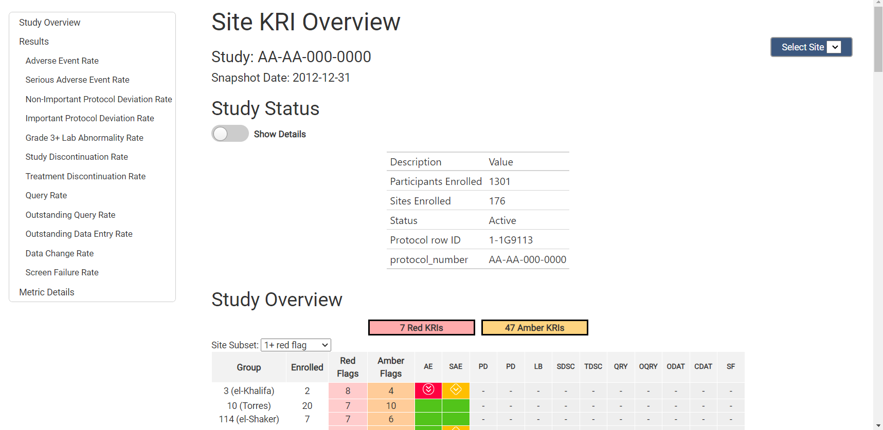
strOutputFile = "test_kri_report.html")Below, you will see a screenshot from the beginning of the report. All charts for all metrics that were included throughout the analysis and reporting workflows will be included in this report.
Using YAML Workflows to generate reports
While it is helpful to understand how each step of this process works, we have provided a series of YAML workflow files that make running reports on multiple KRIs easy and with the ability to be automated.
Here, you will see two options for how to run your workflows. The
first is to run the analytics workflow(s), followed by the reporting
workflow data_reporting.yaml followed by the charts and
reports workflow reports.yaml. This allows the user to
examine the output of each workflow individually before moving on to the
next step.
The second option is to run the snapshot.yaml workflow,
which takes in all raw data (including site and study data) and a few
extra metadata arguments at the beginning of the workflow, and the
result is a list with all data frames and charts from both models, as
well as a report html saved to your working directory.
Option 1 - Run All Workflows Separately
# Step 1 - Create Mapped Data - filter/map raw data
# Source Data
lSource <- list(
    Source_SUBJ = clindata::rawplus_dm,
    Source_AE = clindata::rawplus_ae,
    Source_PD = clindata::ctms_protdev,
    Source_LB = clindata::rawplus_lb,
    Source_STUDCOMP = clindata::rawplus_studcomp,
    Source_SDRGCOMP = clindata::rawplus_sdrgcomp %>% dplyr::filter(.data$phase == 'Blinded Study Drug Completion'),
    Source_DATACHG = clindata::edc_data_points,
    Source_DATAENT = clindata::edc_data_pages,
    Source_QUERY = clindata::edc_queries,
    Source_ENROLL = clindata::rawplus_enroll,
    Source_SITE = clindata::ctms_site,
    Source_STUDY = clindata::ctms_study
)

# Step 0 - Data Ingestion - standardize tables/columns names
lRaw <- list(
    Raw_SUBJ = lSource$Source_SUBJ,
    Raw_AE = lSource$Source_AE,
    Raw_PD = lSource$Source_PD %>%
      dplyr::rename(subjid = subjectenrollmentnumber),
    Raw_LB = lSource$Source_LB,
    Raw_STUDCOMP = lSource$Source_STUDCOMP,
    Raw_SDRGCOMP = lSource$Source_SDRGCOMP,
    Raw_DATACHG = lSource$Source_DATACHG %>%
      dplyr::rename(subject_nsv = subjectname),
    Raw_DATAENT = lSource$Source_DATAENT %>%
      dplyr::rename(subject_nsv = subjectname),
    Raw_QUERY = lSource$Source_QUERY %>%
      dplyr::rename(subject_nsv = subjectname),
    Raw_ENROLL = lSource$Source_ENROLL,
    Raw_SITE = lSource$Source_SITE %>%
      dplyr::rename(studyid = protocol) %>%
      dplyr::rename(invid = pi_number) %>%
      dplyr::rename(InvestigatorFirstName = pi_first_name) %>%
      dplyr::rename(InvestigatorLastName = pi_last_name) %>%
      dplyr::rename(City = city) %>%
      dplyr::rename(State = state) %>%
      dplyr::rename(Country = country),
    Raw_STUDY = lSource$Source_STUDY %>%
      dplyr::rename(studyid = protocol_number) %>%
      dplyr::rename(Status = status)
)

# Step 1 - Create Mapped Data Layer - filter, aggregate and join raw data to create mapped data layer
mappings_wf <- MakeWorkflowList(strPath = "workflow/1_mappings")
mapped <- RunWorkflows(mappings_wf, lRaw)

# Step 2 - Create Metrics - calculate metrics using mapped data
metrics_wf <- MakeWorkflowList(strPath = "workflow/2_metrics")
analyzed <- RunWorkflows(metrics_wf, mapped)

# Step 3 - Create Reporting Layer - create reports using metrics data
reporting_wf <- MakeWorkflowList(strPath = "workflow/3_reporting")
reporting <- RunWorkflows(reporting_wf, c(mapped, list(lAnalyzed = analyzed, lWorkflows = metrics_wf)))

# Step 4 - Create KRI Reports - create KRI report using reporting data
module_wf <- MakeWorkflowList(strPath = "workflow/4_modules")
lReports <- RunWorkflows(module_wf, reporting)

#### 3.2 - Automate data ingestion using Ingest() and CombineSpecs()
# Step 0 - Data Ingestion - standardize tables/columns names
mappings_wf <- MakeWorkflowList(strPath = "workflow/1_mappings")
mappings_spec <- CombineSpecs(mappings_wf)
lRaw <- Ingest(lSource, mappings_spec)

# Step 1 - Create Mapped Data Layer - filter, aggregate and join raw data to create mapped data layer
mapped <- RunWorkflows(mappings_wf, lRaw)

# Step 2 - Create Metrics - calculate metrics using mapped data
metrics_wf <- MakeWorkflowList(strPath = "workflow/2_metrics")
analyzed <- RunWorkflows(metrics_wf, mapped)

# Step 3 - Create Reporting Layer - create reports using metrics data
reporting_wf <- MakeWorkflowList(strPath = "workflow/3_reporting")
reporting <- RunWorkflows(reporting_wf, c(mapped, list(lAnalyzed = analyzed, lWorkflows = metrics_wf)))

# Step 4 - Create KRI Report - create KRI report using reporting data
module_wf <- MakeWorkflowList(strPath = "workflow/4_modules")
lReports <- RunWorkflows(module_wf, reporting)
Recap - Reporting Workflow
-
dfGroupscreated from CTMS data usingRunQuery(),MakeLongMeta()andbind_rows() -
dfMetricscreated fromlWorkflowusingMakeMetric() -
dfResultscreated fromlAnalysis$dfSummaryusingBindResults() -
dfBoundscreated fromdfResultsusingMakeBounds() - List of all charts and tables (
lCharts) created fromdfResults,dfBounds,dfMetricsanddfGroupsusingMakeCharts() - Report generated from
lCharts,dfResults,dfMetricsanddfGroupsusingReport_KRI()
Appendix 1 - Supporting Functions
Mapping Functions
-
RunQuery(): Run a SQL query to create new data.frames with filtering and column name specifications.
Visualization Functions
-
Visualize_Scatter(): Creates scatter plot of Total Exposure (in days, on log scale) vs Total Number of Event(s) of Interest (on linear scale). Each data point represents one site. Outliers are plotted in red with the site label attached. This plot is only created when statistical method is not defined asidentity. Chart is calledscatterin thelChartsobject. -
Visualize_Score(): Provides a standard visualization for Score or KRI. Charts are calledbarScoreorbarMetricin thelChartsobject. -
Visualize_Metric(): Creates all available charts and tables for a metric using the data provided.
Widget Functions
-
Widget_GroupOverview(): Creates an interactive table displaying the flag distribution for all groups across all metrics. -
Widget_BarChart(): Creates an interactive bar chart visualization for Score or KRI. Charts are calledbarScoreJSorbarMetricJSin thelChartsobject. -
Widget_ScatterPlot(): Creates an interactive scatter plot of Total Exposure (in days, on log scale) vs Total Number of Event(s) of Interest (on linear scale). Each data point represents one site. Outliers are plotted in red with the site label attached.Chart is calledscatterJSin thelChartsobject. -
Widget_TimeSeries(): Creates an interactive time series scatter plot of the score, metric or numerator. Charts are calledtimeSeriesContinuousScoreJS,timeSeriesContinuousMetricJS, ortimeSeriesContinuousNumeratorJSin thelChartsobject.
Table Functions
-
Report_MetricTable(): Creates a sortable table displaying the flags per group (e.g. Site, Country) for one metric at a time.