S3 plot method for class initial_graph — plot.initial

The plot of an initial_graph translates the hypotheses into vertices and transitions into edges to create a network plot. Vertices are labeled with hypothesis names and hypothesis weights, and edges are labeled with transition weights. See vignette("graph-examples") for more illustration of commonly used multiple comparison procedure using graphs.

Usage

# S3 method for class 'initial_graph'
plot(
  x,
  ...,
  v_palette = c("#6baed6", "#cccccc"),
  layout = "grid",
  nrow = NULL,
  ncol = NULL,
  edge_curves = NULL,
  precision = 4,
  eps = NULL,
  background_color = "white",
  margins = c(0, 0, 0, 0)
)

Arguments

x: An object of class initial_graph to plot.
...: Other arguments passed on to igraph::plot.igraph().
v_palette: A character vector of length two specifying the colors for retained and deleted hypotheses. More extensive color customization must be done with vertex.color.
layout: An igraph layout specification (See ?igraph.plotting), or "grid", which lays out hypotheses left-to-right and top-to-bottom. nrow and ncol control the grid shape.
nrow: An integer scalar specifying the number of rows in the vertex grid. If row and column counts are not specified, vertices will be laid out as close to a square as possible.
ncol: An integer scalar specifying the number of columns in the vertex grid. If row and column counts are not specified, vertices will be laid out as close to a square as possible.
edge_curves: A named numeric vector specifying the curvature of specific edges. Edge pairs (Where two vertices share an edge in each possible direction) are detected automatically and get 0.25 curvature. Adjust edges by adding an entry with name "vertex1|vertex2, and adjust default edge pairs curvature by adding an entry with name "pairs" - edge_curves = c("pairs" = 0.5, "H1|H3" = 0.25, "H3|H4" = 0.75).
precision: An integer scalar indicating the number of decimal places to to display.
eps: A numeric scalar. The transition weight of eps will be displayed as \(\epsilon\), which indicates edges with infinitesimally small weights. See Bretz et al. (2009) for more details.
background_color: A character scalar specifying a background color for the whole plotting area. Passed directly to graphics::par() (bg).
margins: A length 4 numeric vector specifying the margins for the plot. Defaults to all 0, since igraph plots tend to have large margins. It is passed directly to graphics::par() (mar).

Value

An object x of class initial_graph, after plotting the initial graph.

Customization of graphs

There are a few values for igraph::plot.igraph() that get their defaults changed for graphicalMCP. These values can still be changed by passing them as arguments to plot.initial_graph(). Here are the new defaults:

vertex.color = "#6baed6",
vertex.label.color = "black",
vertex.size = 20,
edge.arrow.size = 1,
edge.arrow.width = 1,
edge.label.color = "black"
asp = 0.

Neither graphicalMCP nor igraph does anything about overlapping edge labels. If you run into this problem, and vertices can't practically be moved enough to avoid collisions of edge labels, using edge curves can help. igraph puts edge labels closer to the tail of an edge when an edge is straight, and closer to the head of an edge when it's curved. By setting an edge's curve to some very small value, an effectively straight edge can be shifted to a new position.

References

Bretz, F., Posch, M., Glimm, E., Klinglmueller, F., Maurer, W., and Rohmeyer, K. (2011). Graphical approaches for multiple comparison procedures using weighted Bonferroni, Simes, or parametric tests. Biometrical Journal, 53(6), 894-913.

Xi, D., and Bretz, F. (2019). Symmetric graphs for equally weighted tests, with application to the Hochberg procedure. Statistics in Medicine, 38(27), 5268-5282.

Examples

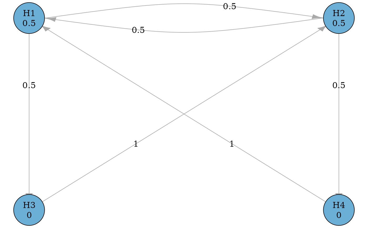
# A graphical multiple comparison procedure with two primary hypotheses (H1
# and H2) and two secondary hypotheses (H3 and H4)
# See Figure 4 in Bretz et al. (2011).
hypotheses <- c(0.5, 0.5, 0, 0)
delta <- 0.5
transitions <- rbind(
  c(0, delta, 1 - delta, 0),
  c(delta, 0, 0, 1 - delta),
  c(0, 1, 0, 0),
  c(1, 0, 0, 0)
)
g <- graph_create(hypotheses, transitions)
plot(g)


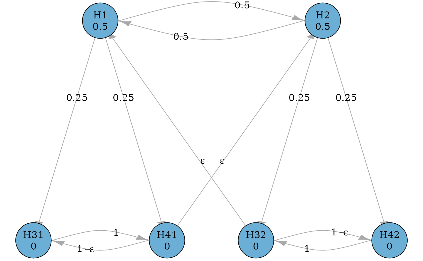
# A graphical multiple comparison procedure with two primary hypotheses (H1
# and H2) and four secondary hypotheses (H31, H32, H41, and H42)
# See Figure 6 in Xi and Bretz (2019).
hypotheses <- c(0.5, 0.5, 0, 0, 0, 0)
epsilon <- 1e-5
transitions <- rbind(
  c(0, 0.5, 0.25, 0, 0.25, 0),
  c(0.5, 0, 0, 0.25, 0, 0.25),
  c(0, 0, 0, 0, 1, 0),
  c(epsilon, 0, 0, 0, 0, 1 - epsilon),
  c(0, epsilon, 1 - epsilon, 0, 0, 0),
  c(0, 0, 0, 1, 0, 0)
)
hyp_names <- c("H1", "H2", "H31", "H32", "H41", "H42")
g <- graph_create(hypotheses, transitions, hyp_names)

plot_layout <- rbind(
  c(0.15, 0.5),
  c(0.65, 0.5),
  c(0, 0),
  c(0.5, 0),
  c(0.3, 0),
  c(0.8, 0)
)

plot(g, layout = plot_layout, eps = epsilon, edge_curves = c(pairs = .5))