Rationales to generate the closure and the weighting strategy of a graph • graphicalMCP

Motivating example

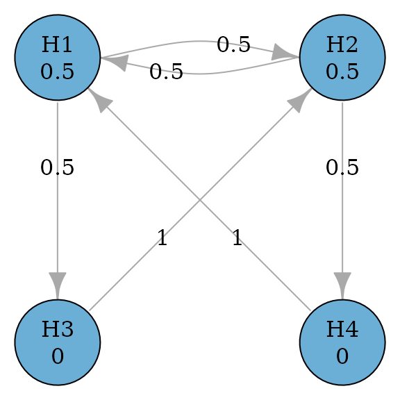
Consider a simple successive graph with four hypotheses. It has two primary hypotheses $H_1$ and $H_2$ and two secondary hypotheses $H_3$ and $H_4$ . Initially, hypothesis weights are split equally between $H_1$ and $H_2$ with 0.5. Hypotheses $H_3$ and $H_4$ receive 0 hypothesis weights because $H_3 (H_4)$ is tested only if $H_1 (H_2)$ is rejected. Thus there is an edge from $H_1 (H_2)$ to $H_3 (H_4)$ with a transition weight of 1. When both $H_1$ and $H_3$ are rejected, their hypothesis weights are propagated to $H_2$ ; similarly, when both $H_2$ and $H_4$ are rejected, their hypothesis weights are propagated to $H_1$ . Thus there is an edge from $H_3 (H_4)$ to $H_2 (H_1)$ with a transition weight of 1. A graphical multiple comparison procedure is illustrated below.

Generating the closure

The closure of this multiple comparison procedure is a collection of intersection hypotheses $H_1\cap H_2\cap H_3\cap H_4$ , $H_1\cap H_2\cap H_3$ , $H_1\cap H_2\cap H_4$ , $H_1\cap H_3\cap H_4$ , $H_2\cap H_3\cap H_4\ \ldots, H_1, H_2, H_3$ , and $H_4$ . In other words, these intersection hypotheses consist of intersections based on all non-empty subsets of $\{1, 2, 3, 4\}$ , e.g., $\{1, 2, 3\}$ , $\{1, 2, 4\}$ , $\{1, 3, 4\}$ , $\{2, 3, 4\}$ , $\ldots$ . Thus there are $2^4-1$ intersection hypotheses. An equivalent way to generate all intersection hypotheses is to use a binary representation. For example, the intersection hypothesis $H_1\cap H_2\cap H_3\cap H_4$ corresponds to $(1, 1, 1, 1)$ and $H_1\cap H_2\cap H_3$ corresponds to $(1, 1, 1, 0)$ . Then the closure can be indexed by the power set of $\{1, 2, 3, 4\}$ as below. In general, one can use rev(expand.grid(rep(list(1:0), m))) to general the closure, where $m$ is the number of hypotheses.

#>    H1 H2 H3 H4
#> 1   1  1  1  1
#> 2   1  1  1  0
#> 3   1  1  0  1
#> 4   1  1  0  0
#> 5   1  0  1  1
#> 6   1  0  1  0
#> 7   1  0  0  1
#> 8   1  0  0  0
#> 9   0  1  1  1
#> 10  0  1  1  0
#> 11  0  1  0  1
#> 12  0  1  0  0
#> 13  0  0  1  1
#> 14  0  0  1  0
#> 15  0  0  0  1

Calculating the weighting strategy

Given the closure, one can calculate the hypothesis weight associated with every hypothesis in every intersection hypothesis using Algorithm 1 (Bretz et al. 2011). The whole collection of hypothesis weights is called a weighting strategy. For example, hypothesis weights are $(0.5, 0.5, 0, 0)$ for the intersection hypothesis $H_1\cap H_2 \cap H_3\cap H_4$ . Then hypothesis weights for the intersection hypothesis $H_1\cap H_2 \cap H_3$ are $(0.5, 0.5, 0, 0)$ , which can be calculated by removing $H_4$ from the initial graph and applying Algorithm 1 (Bretz et al. 2011). The algorithm calculates hypothesis weights in a step-by-step fashion. For example, for the intersection hypothesis $H_1\cap H_2$ , it can start from $H_1\cap H_2 \cap H_3\cap H_4$ and calculates hypothesis weights for $H_1\cap H_2 \cap H_3$ by removing $H_4$ and then calculates hypothesis weights for $H_1\cap H_2$ by removing $H_3$ ; it can also start from $H_1\cap H_2 \cap H_3$ (assuming its hypotheses weights are stored) and calculates hypothesis weights for $H_1\cap H_2$ by removing $H_3$ . Therefore, there are two strategies to calculate the weighting strategy.

#>      H1   H2   H3   H4
#> 1  0.50 0.50 0.00 0.00
#> 2  0.50 0.50 0.00 0.00
#> 3  0.50 0.50 0.00 0.00
#> 4  0.50 0.50 0.00 0.00
#> 5  0.75 0.00 0.00 0.25
#> 6  1.00 0.00 0.00 0.00
#> 7  0.75 0.00 0.00 0.25
#> 8  1.00 0.00 0.00 0.00
#> 9  0.00 0.75 0.25 0.00
#> 10 0.00 0.75 0.25 0.00
#> 11 0.00 1.00 0.00 0.00
#> 12 0.00 1.00 0.00 0.00
#> 13 0.00 0.00 0.50 0.50
#> 14 0.00 0.00 1.00 0.00
#> 15 0.00 0.00 0.00 1.00

Approach 1: Simple approach

The first strategy utilizes the initial graph as the starting point and calculates hypothesis weights for all other intersection hypotheses. For example, to calculate hypothesis weights for $H_1\cap H_2$ , it will start with the intersection hypothesis $H_1\cap H_2 \cap H_3\cap H_4$ and sequentially remove $H_4$ and $H_3$ (or in the other order). This approach is simple to implement since hypothesis weights for $H_1\cap H_2 \cap H_3\cap H_4$ are determined by the initial graph and always available. This approach is similar to the one implemented in the gMCP R package. The drawback is that it does not use other information to reduce the number of calculations. For example, it is possible that hypothesis weights for $H_1\cap H_2 \cap H_3$ have been calculated when calculating for $H_1\cap H_2$ . Using the information from $H_1\cap H_2 \cap H_3$ would only need the one-step calculation, compared to the two-step calculation using $H_1\cap H_2 \cap H_3\cap H_4$ .

Approach 2: Parent-child approach

This approach tries to avoid the drawback of Approach 1 by saving intermediate graphs. Then it only performs one-step calculation which could save time. In general, an intersection hypothesis has a parent intersection hypothesis, which involves all hypotheses involved in the first intersection and has one extra hypothesis. For example, the second row of matrix_intersections is $H_1\cap H_2 \cap H_3$ and its parent intersection is $H_1\cap H_2 \cap H_3\cap H_4$ in the first row; the third row of matrix_intersections is $H_1\cap H_2 \cap H_4$ and its parent intersection is $H_1\cap H_2 \cap H_3\cap H_4$ in the first row. Thus we can identify the parent intersection hypothesis for each row in matrix_intersections (except row 1) as the row number 1, 1, 2, 1, 2, 3, 4, 1, 2, 3, 4, 5, 6, 7. Given this sequence of parent hypotheses, it is simple to obtain hypothesis weights for an intersection hypothesis based on its parent intersection hypothesis via one-step calculation.

It is of interest to understand this pattern and obtain it efficiently. First, between the bottom half (rows 9 - 15) and top half (rows 1 - 7), each row’s parent in the bottom half is the corresponding row in the top half, eight rows up, because the only difference is the flipping of $H_1$ from 1 in the top half to 0 in the bottom half. For example, row 15’s parent is in row 15 - 8 = 7. Using this observation, we can determine parent hypotheses for rows from 9 to 15 as 1, 2, 3, 4, 5, 6, 7. A similar pattern can be observed for rows from 5 to 8. Their parent hypotheses are in rows 1, 2, 3, 4, respectively, by flipping $H_2$ from 1 to 0. For rows 3 - 4, their parent hypotheses are in rows 1, 2, respectively, by flipping $H_3$ from 1 to 0. Lastly for row 2, its parent hypothesis is in row 1. The row number of the parent hypothesis can be efficiently generated by running do.call(c, lapply(2^(seq_len(m) - 1), seq_len))[-2^m, ], where $m$ is the number of hypotheses.

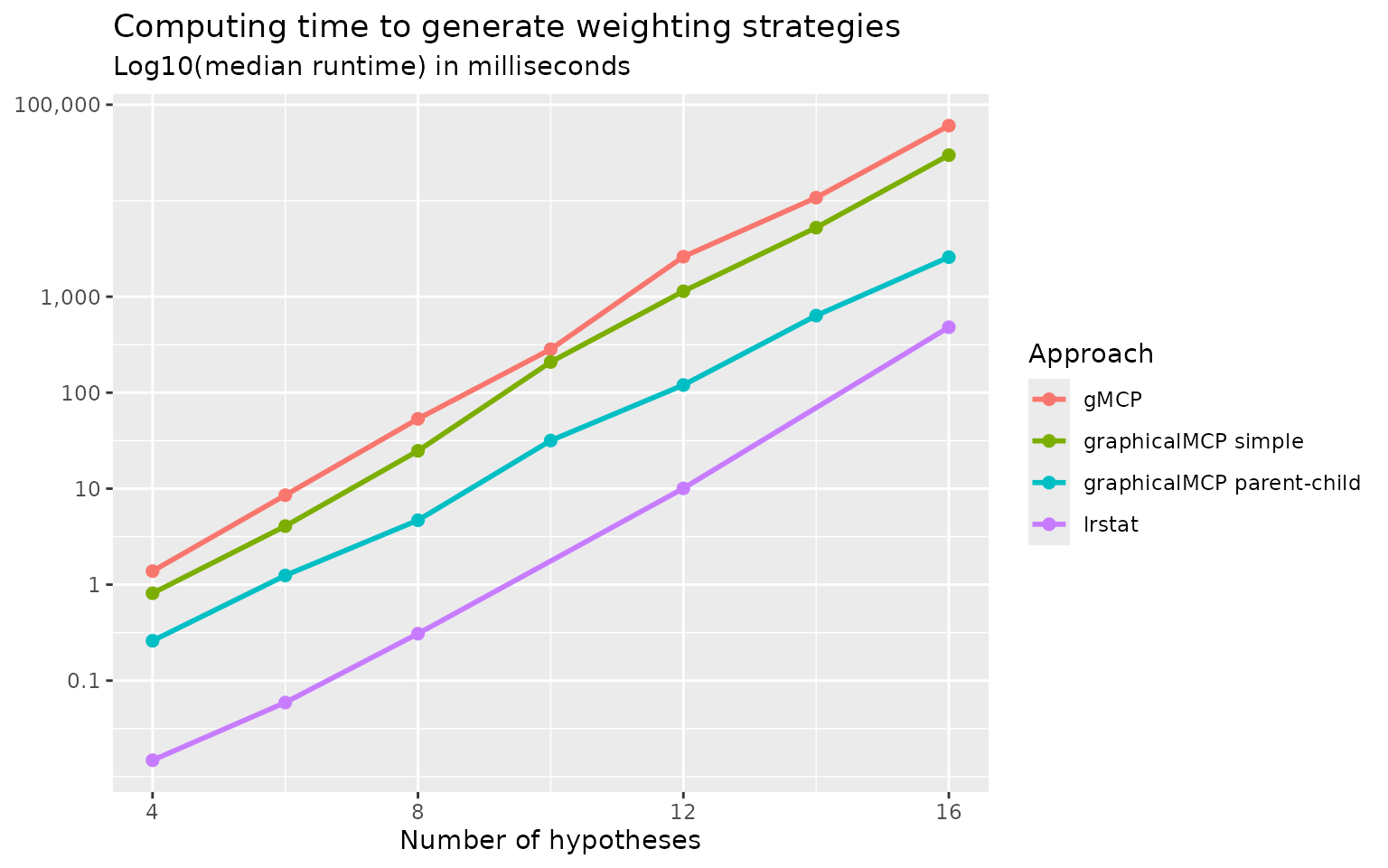
Comparing different approaches to calculating weighting strategies

To benchmark against existing approaches to calculating weighting strategies, we compare the following approaches: gMCP::generateWeights() (Rohmeyer and Klinglmueller 2024), lrstat::fwgtmat() (Lu 2016), Approach 1 (graphicalMCP simple) and Approach 2 (graphicalMCP parent-child). Random graphs are generated for the numbers of hypotheses of 4, 8, 12, and 16. Computing time (in median log-10 milliseconds) is plotted below. We can see that gMCP::generateWeights() is the slowest and lrstat::fwgtmat() is the fastest. Approach 2 (graphicalMCP parent-child) is faster than Approach 1 (graphicalMCP simple). Note that lrstat::fwgtmat() implements the calculation using C++, which is known to be faster than R. But it is less stable than other approaches, e.g., giving errors more often than others. Given that the computing time of R-based approaches is acceptable, adding Rcpp dependency is not considered in graphicalMCP. For these considerations, we implement Approach 2 in graphicalMCP::graph_generate_weights().

Improving power simulations using parent-child relationships

Conventional approach for power simulations

The conventional approach for power simulations is to repeat the following process many times, e.g., 100,000 times.

Simulate a set of p-values
Run the graphical multiple comparison procedure to
- Determine which hypothesis can be rejected
- Remove the rejected hypothesis and update the graph
- Repeat until no more hypotheses can be rejected

Note that the same step to update the graph may repeat in many replications, which may be repetitive. For $m$ hypotheses, there are at most $2^m-1$ graphs depending on which hypotheses are rejected. These graphs correspond to the closure and the weighting strategy. Thus an idea to avoid redundant updating of graphs is to utilize the weighting strategy.

Power simulations using parent-child relationships

The key to allow this approach is to efficiently identify the row of the weighting strategy, given which hypotheses are rejected. Remembering the pattern we found for Approach 2, the bottom half (rows 9 - 15) of matrix_intersections is the same as the top half (rows 1 - 7), except flipping $H_1$ from 1 to 0. This means that if $H_1$ has not been rejected (1 for $H_1$ in matrix_intersections), the row number of that index should be in the top half. For example, assume that $H_2$ and $H_4$ have been rejected and the index in matrix_intersections should be $(1, 0, 1, 0)$ . Since $H_1$ is 1, the corresponding row should be in the top half (rows 1- 7). But $H_2$ is 0 and thus the corresponding row should be in the bottom half within the top half (rows 5 - 7). Since $H_3$ is 1 and thus the corresponding row should be in the top half (rows 5 - 6). But $H_4$ is 0 and thus the corresponding row should be 6. A useful way to calculate the row number for an index of XXXX is 2^m - sum(XXXX * 2^(m:1 - 1)). For example for XXXX=1010, its row number should be (1 - 1) * 8 + (1 - 0) * 4 + (1 - 1) * 2 + (1 - 0) * 1 + 1 = 16 - 10 = 6.

With the above way of efficiently identifying rows of weighting_strategy, power simulations could be implemented as follows:

Obtain the weighting strategy (once for all simulations)
Simulate a set of p-values
Run the graphical multiple comparison procedure to
- Determine which hypothesis can be rejected
- Remove the rejected hypothesis and identify the row of the weighting strategy
- Repeat until no more hypotheses can be rejected

The small modification in Step 3b makes this approach much faster than the conventional approach for power simulations.

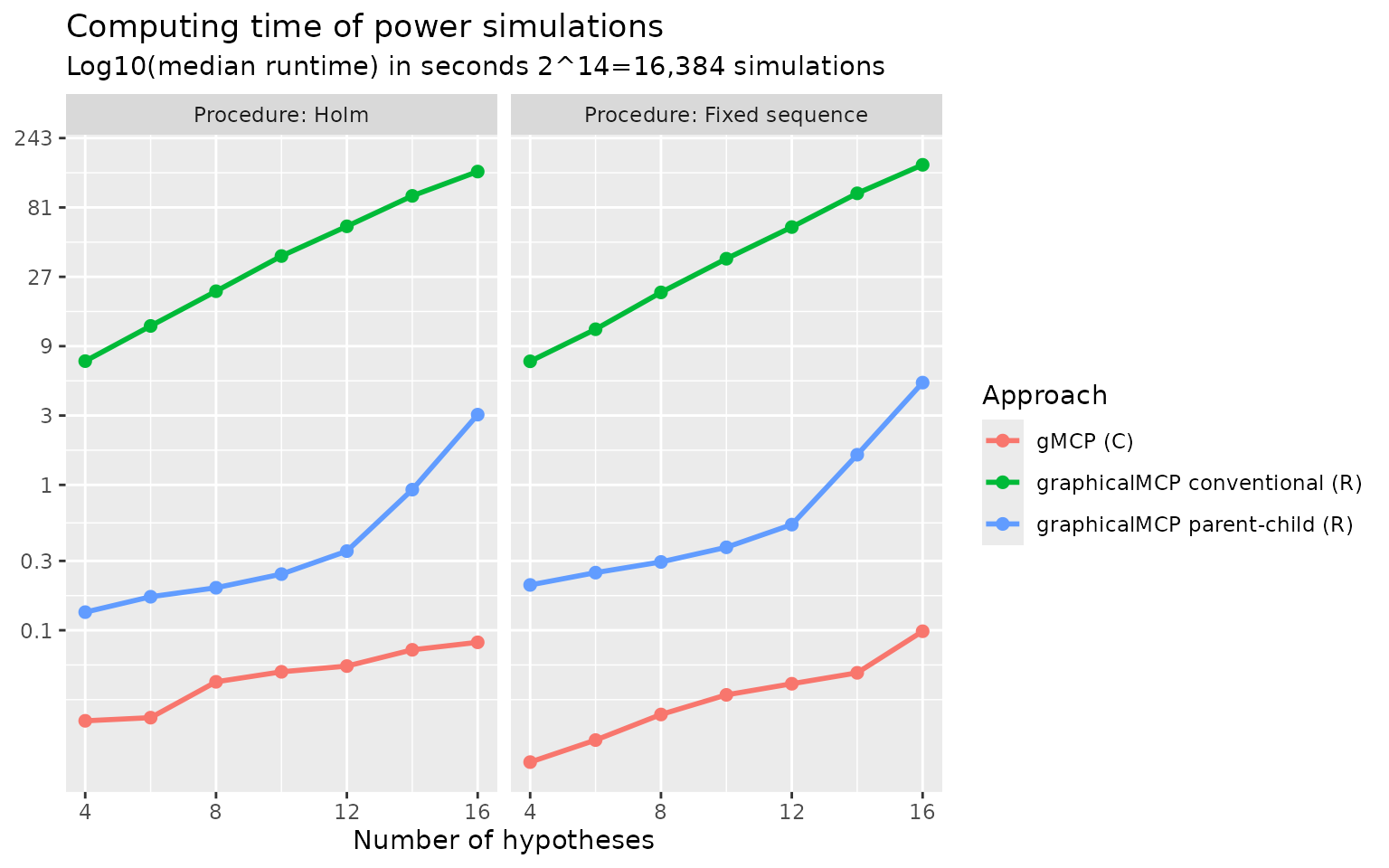
Comparing different approaches to power simulations

To benchmark against existing approaches to calculating weighting strategies, we compare the following approaches: gMCP::calcPower(), Approach 1 (graphicalMCP conventional), and Approach 2 (graphicalMCP parent-child). Both Holm and fixed sequence procedures are considered with the numbers of hypotheses of 4, 8, 12, and 16. Computing time (in median log-10 seconds) is plotted below. We can see that gMCP::calcPower() is the fastest and Approach 1 (graphicalMCP conventional) is the lowest. Note that gMCP::calcPower() implements the simulation using C, which is known to be faster than R but is not easy to extend to other situations. Given that the computing time of Approach 2 (graphicalMCP parent-child) is acceptable, we implement it in graphicalMCP::graph_calculate_power().

Reference

Bretz, Frank, Martin Posch, Ekkehard Glimm, Florian Klinglmueller, Willi Maurer, and Kornelius Rohmeyer. 2011. “Graphical Approaches for Multiple Comparison Procedures Using Weighted Bonferroni, Simes, or Parametric Tests.” Biometrical Journal 53 (6): 894–913. https://onlinelibrary.wiley.com/doi/10.1002/bimj.201000239.

Lu, Kaifeng. 2016. “Graphical Approaches Using a Bonferroni Mixture of Weighted Simes Tests.” Statistics in Medicine 35 (22): 4041–55. https://onlinelibrary.wiley.com/doi/10.1002/sim.6985.

Rohmeyer, Kornelius, and Florian Klinglmueller. 2024. gMCP: Graph Based Multiple Test Procedures. https://cran.r-project.org/package=gMCP.